Dynamic Asset Allocation for Practitioners Part 1: The Many Faces of Momentum

A (Very) Short History of Dynamic Asset Allocation

The field of tactical or dynamic asset allocation has grown dramatically since Mebane Faber published what is perhaps the first broadly accessible paper on the topic in 2007, 'A Quantitative Approach to Tactical Asset Allocation'. Faber's original paper utilized a simple 10 month moving average as a signal to move into or out of a basket of 5 major global asset classes. Over the period 1970 through the paper's 2009 update, this technique generated better returns than any of the individual assets in the sample universe - U.S. and EAFE stocks, U.S. real estate, Treasuries and commodities - and with substantially lower risk than the equal weight basket or a 60/40 stock/Treasury portfolio.

In 2009 Faber published a follow-up paper called 'Relative Strength Strategies for Investing' which introduced the concept of price momentum as a way to distinguish between strong and weak assets in the portfolio. That paper applied an intuitive method of capturing asset class momentum that involved averaging each asset's rate of change (ROC) across five lookback horizons, specifically 1, 3, 6, 9 and 12 months. By averaging across lookback horizons, this approach captures momentum at multiple periodicities, and also identifies acceleration by implicitly weighting near-term price moves more heavily than price moves at longer horizons.

In May of 2012 we published a whitepaper entitled, "Adaptive Asset Allocation: A Primer", a quantitative systematic methodology integrating the simple ROC based momentum concepts introduced in Faber's 'Relative Strength' paper with techniques derived from the portfolio optimization literature. Specifically, the paper explained how applying a minimum variance optimization overlay to a portfolio of high momentum assets serves to stabilize and strengthen both absolute and risk-adjusted portfolio performance.

Article Series

We are going to range far and wide in our exploration of global dynamic asset allocation. This article, the first in our series, will explore a variety of methods to rank assets based on price momentum. The second article will introduce several approaches to rank assets based on risk-adjusted momentum measures. The third article will introduce a framework for thinking about portfolio optimization, including several heuristic and formal optimization methods.

Our fourth article will discuss ways of combining the best facets of momentum with the best techniques for portfolio optimization to offer a coherent framework for global dynamic asset allocation. The objective here will be robustness and logical coherence rather than utilizing optimization for best in-sample simulation performance. 

Lastly, we are considering introducing some ensemble concepts and adaptive frameworks as a cherry on top, but we aren't sure how far we want to go yet, so we'll just get started and see where it takes us.

The following illustrates the proposed framework for this article series:

Methodology

This first article will explore a variety of methods for identifying trend strength for asset allocation, with the goal of comparing and contrasting the various methods under different assumptions of portfolio concentration and asset universe specifications.

We take the position that portfolio concentration is a source of potential data mining bias because the results for dynamic asset allocation approaches can vary widely depending on the number of top assets that are held in the portfolio at each rebalance. Some approaches do better with more concentration, and others with less. We will test with concentrations of top 2, 3, 4 and 5 assets and average the results.

The asset universe can serve as a source of potential 'curve fitting' as well, as it is easy and compelling to want to remove assets from the universe that drag down returns in simulation, or add assets with strong results over the backtest horizon.

To avoid this trap, we run our simulations on a diversified universe of 10 global asset classes, as well as ten other asset universes where we drop one of the ten original assets. This helps to control for the chance that strong performance is simply the result of one dominant asset class over the period.

The ten asset classes we will use for all testing are:

• Commodities (DB Liquid Commoties Index)
• Gold
• U.S. Stocks (Fama French top 30% by market capitalization)
• European Stocks (Stoxx 350 Index)
• Japanese Stocks (MSCI Japan)
• Emerging Market Stocks (MSCI EM)
• U.S. REITs (Dow Jones U.S. Real Estate Index)
• International REITs (Dow Jones Int'l Real Estate Index)
• Intermediate Treasuries (Barclays 7-10 Year Treasury Index)
• Long Treasuries (Barclays 20+ Year Treasury Index)

Importantly, this article is NOT about parameter optimization; for all tests we use the exact same lookback parameter lengths (where applicable) to avoid the distraction of searching for a priori local parameter optima which will almost certainly NOT prove to be true optima out of sample.

It is important to decide how we will evaluate the relative efficacy of the various approaches before we start testing. For each strategy we will show the average statistics for all simulations with 2, 3, 4, and 5 holdings, and across all 11 asset universes. Recall that we are testing the full 10 asset class universe, as well as 10 other 9 asset class universes where one of the original assets is removed. So the statistics for each strategy will actually represent an average (median) of 44 simulations (4 portfolio concentrations x 11 universes). We will then present modified histograms to illustrate the range of outcomes for each strategy. This represents a rare test of robustness across methodologies.

Toward the bottom of this article, we demonstrate how combining all of the indicators into a naive ensemble delivers better performance than any of them individually.

Momentum Metrics

For the purpose of this article we used 8 indicators for measuring trend strength. All of the metrics rank assets at monthly rebalance periods based on an average of values observed over the lookback windows described above, which were chosen to be consistent with Mebane Faber's original momentum paper.

The intuition behind testing a variety of momentum techniques relates to the ability of different measures to stabilize the estimate using simple or advanced ensemble process.

The following list describes the mechanics of each method of momentum calculation, where t is the current date, n is the lookback parameter, and N is the number of assets in the testing universe. Note that each indicator is calculated at each of the 5 lookbacks, and then the indicators are averaged across lookbacks to generate the final measure.

• Total return - this is the most common measure of momentum, where assets are ranked on their historical total returns.
  
  
  
  
  
• SMA Differential - this technique uses the differential between a shorter term and longer term moving average as the momentum measure. We used our standard parameters to define the length of the longer SMAs. The length of corresponding short SMAs was simply 1/10th of the length of the longer SMA. So for example, for the 120 day parameter, we measured the differential between the 120 day SMA and the 12 day SMA.
  
  
  
  
  
• Price to SMA Differential - similar to SMA Differential, except that this technique uses the differential between the current price and the n-day SMA rather than using a shorter moving average. 
  
  
  
  
  
• SMA Instantaneous Slope - For this metric we derived the instantaneous slope of each moving average. Essentially this measures the rate of change of each SMA using the difference between yesterday's SMA and today's SMA.
  
  
  
  
  
• Price Percent Rank - This metric captures the location of the current price relative to the security's range over each lookback period. The lowest price over the period would have a rank of 1, while the highest would have a rank of 100. The median price over the period would have a rank of 50.
  
  
  
• Z-Score - Analogous to the Price Percent Rank, z-score captures the magnitude that the current price deviates from the average price over the period.
  
  
  
• Z-Distribution - This method transforms the z-score to a percentile value on the cumulative normal distribution. Under this framework the trend strength measure will accelerate in magnitude as the price strays further away from the mean. The function to perform this translation is complicated, but it can be easily generated in Excel using the Norm.S.Dist(z, TRUE) function.
  
  
  
  
  
• T-Distribution - The normal distribution is valid when the sample size is large enough so that the sample is likely to be representative of the population. Under conditions where the sample size is small and the parameters that describe the distribution are unknown, a more appropriate choice is the Student's t-distribution. The t-distribution transforms a t-score into a percentile given the number of degrees of freedom. The degrees of freedom are equal to (n - 1).
  
  
  
  
  

It is worth noting that the SMA-differential approaches described above are related to typical moving average crossover systems applied in trend following. The critical difference in our proposed framework is that, unlike trend following approaches, which measure the 'state' of a trend, our momentum indicators measure the 'strength' of a trend. Crossover systems are either long or short (triple crossovers can be neutral too), which means they are 'binary' variables, whereas the momentum indicators provide discrete variables that allow us to compare the relative strength of the trends. 

Importantly, because we measure trend strength across five lookback time horizons, the cross sectional measure of price momentum needs to be standardized. It is silly to average an annualized 20 day ROC with a 250 day ROC because the 20 day ROC will deliver much more extreme values, on average, than the 250 day ROC, and will dominate the momentum measure commensurately.

There are a number of ways to standardize the momentum measure across lookbacks, but the method we used was to calculate each asset's proportion of total absolute cross sectional momentum across all assets over each lookback horizon, holding the sign constant.

Again, standardized momentum scores are then averaged across all lookbacks to determine the final momentum score for each asset.

Results

Table 1. displays the salient statistics for tests of each of the momentum methods (indicators) described above. Each cell describes the median performance across all 44 combinations (holding 2 - 5 positions, 11 universe combinations) that we tested for each methodology. 

Chart 1. Median performance summary

Data sources: Bloomberg

The instantaneous slope method seems to deliver the best median performance statistics all around, with the highest overall returns, the highest Sharpe, and the lowest median Maximum Drawdown of all methods. But the median is just one point on the distribution; let's see what the range of outcomes looks like for each system.

Performance Distribution

Charts 1 through 9 below show all 44 of the equity lines (4 concentrations x 11 universe combinations) that were used to calculate the median performance measures in Table 1 for each momentum indicator. The first highlighted chart shows all 352 equity lines derived from all 44 portfolio combinations across all 8 indicators.

Charts 1 - 9: Equity lines for indicators across 44 universe/concentration combinations

Source: Bloomberg

A few observations stand out from these charts. First, they all look a little different, with waves of surges and drawdowns occurring at slightly different times across momentum measures, though all of them show a drawdown in 2008. Second, notice that in some charts the equity lines all cluster together in a narrow range - z-score and instantaneous slope stand out in this respect - while others exhibit quite a wide range of outcomes - price to SMA differential and SMA differential for example.

Charts 10 through 43 below quantify the distribution of return, Sharpe, and Maximum Drawdown outcomes across all 44 versions of each momentum system using a cumulative histogram. In our opinion, the most realistic way to evaluate the performance of a system is on the basis of performance statistics near the bottom of the distribution. The worst outcome could be an outlier, but traditional tests of statistical significance focus on 5th percentile outcomes, so that is where we focus our attention. In each series of charts, we have highlighted the approach with the best results at the 5th percentile.

Charts 10 - 43: Distribution of performance metrics across 44 universe/concentration combinations.

Range of CAGR by Indicator

Source: Bloomberg


Range of Sharpe(0%) by Indicator

Source: Bloomberg


Range of Max Drawdowns by Indicator

Source: Bloomberg

(You will note that the numbers in the 50% column of the charts above are the same as the numbers in Table 1 summary, as the median is simply the 50th percentile value).

Charts 24 through 26 show the average performance of each methodology with portfolio concentrations of 2 holdings through 5 holdings across all 11 asset universes tested. It is interesting to see that, while more concentrated portfolios tend to deliver higher returns, the highest Sharpe ratios are derived from portfolios with 3 or 4 holdings, and these more diversified portfolios tend toward much lower drawdowns as well.

Chart 24. Average indicator returns across 11 asset universe combinations with different portfolio concentration

Source: Bloomberg

Chart 25. Average indicator return/risk ratios across 11 asset universe combinations with different portfolio concentration

 Source: Bloomberg

Chart 26. Average indicator Max Drawdowns across 11 asset universe combinations with different portfolio concentration

Source: Bloomberg

Indicator Diversification

We know from charts 1 - 9 that the different momentum indicators, universe and concentration combinations all deliver slightly different results, where equity rises and falls at slightly different rates. But how different is the performance across indicators really?

Matrix 1. shows the correlations between daily returns for all indicator combinations. The daily returns for all universe and concentration combinations were averaged to generate the final return series for each indicator.

Matrix 1. Pairwise correlations between indicators (average of 44 combinations for each indicator)

Source: Bloomberg

The correlations range from about 0.8 between the t-distribution method and the ROC and instantaneous slope methods, to 0.99 between instantaneous slope and ROC. The average pairwise correlation is 0.936. With correlations so high, to what extent can we take advantage of the different methods to create a diversified system composed of all 352 combinations? Chart 27 and Table 2. give us the answer.

Chart 27. Aggregate Index of all 352 indicator/universe/concentration combinations, equal weight.

Source: Bloomberg


Table 2. Summary statistics for Aggregate Index

Source: Bloomberg

Despite the high average correlations between the different momentum systems, the aggregate equity line provides a material boost to all risk adjusted statistics. While the returns are about 1% below the returns derived from the best individual indicators, the Sharpe(0%) ratio is better than all of them. Further, the average volatility of the 8 individual systems is 12.42%, while the volatility of the aggregate system is the lowest of all at just 11.1%. Lastly, the aggregate system exhibits the lowest drawdowns and the highest percentage of positive rolling 12-month periods.

Obviously it is impractical to run 352 models in parallel, even if they are all closely related. Moreover, this approach is far from the best method to aggregate all of the information from the different indicators; we will touch on different methods of aggregation in our fourth instalment of this series. However, there is clearly value in finding ways to blend various momentum factors to create a more stable allocation model.

Conclusions and Next Steps

In this article we have explored a variety of methods to measure the price momentum of a universe of asset classes for the purpose of creating global dynamic asset allocation models. Given our objective to avoid as much optimization as possible, we tested each momentum method using 4 different levels of portfolio concentration, and 11 slightly modified asset class universes. This approach provided 44 distinct tests for each indicator, which allowed us to investigate the stability of each indicator across parameters. 

Among the individual momentum indicators we tested, the instantaneous slope method delivered the best performance in terms of median returns, Sharpe(0%), drawdowns and percent positive 12-month periods. 

We investigated the impact of different levels of portfolio concentration on performance and discovered, perhaps not surprisingly, that more concentrated portfolios deliver stronger returns, while some diversification does improve risk-adjusted outcomes.

We examined the correlations between the indicator systems and determined that they are all closely related, with average pairwise correlations of about 0.93. However, even with such high average correlations, aggregating the systems into one system composed of all 352 indicator/concentration/ universe combinations delivered the most stable results of all.

Article 2 in our series will perform a similar analysis of several risk-adjusted momentum measures, such as Sharpe ratio, Omega ratio, and Sortino Ratio. As in this article, the Article 2 will hold all portfolio positions in equal weight, but Article 3 will introduce methods to optimize the weights of portfolio holdings to further improve absolute and risk adjusted returns - quite significantly. 

We are just scratching the surface of what is possible with tactical alpha. Chart 27 and Table 3. offer a glimpse of what's to come. Stay tuned.

[Update: Charts and Performance are updated through end of May]

Chart 27. Mystery system

Source: Bloomberg 

Table 3. Mystery system stats

Triumph of the Ostriches

Obviously the title of this post is a riff on the classic book, Triumph of the Optimists by Dimson, Marsh and Staunton (2002). The book describes 100 years of investment returns across a range of markets, making a number of important conclusions. Unsurprisingly, the financial marketing complex narrowly focused its attention on the strong returns the authors observed in equity markets over the post WWII period. 

However, more balanced readers would have noted the authors' belief that the historical indexes analyzed in the book overstate long-term performance because they are contaminated by survivorship bias. The authors are clearly of the opinion that long-term stock returns are seriously overestimated, due to a focus on periods that with hindsight are known to have been successful, while markets that were unsuccessful were not included. In other words, the analysis assumes that an investor would have known which markets would succeed and which would fail in advance.

Many of the most important countries at various stages of the past dozen decades were not included in the study because of a lack of consistent data. For example, Russia, China, Latin America, Eastern Europe and Southeast Asia were all largely ignored. Several of these countries experienced terminal collapses of equity markets and/or bond markets and/or currencies, which explain some of the discontinuities in the data.

Triumph of the Ostriches refers to the current situation in global markets where 'Ostrich' investment managers have been killing it. Recall that (according to the untrue but pervasive myth) an ostrich sticks his head in the sand at any sign of danger; presumably the ostrich perceives that if it doesn't see the danger, then it doesn't exist. In the same way, Ostrich managers ignore any and all signs of market risk in the hope that these risks won't materialize on their watch.

Throwing caution to the wind has been very profitable - so far. But if history is any guide, there are many reasons for investors to consider taking a much more cautious stance.

Here are the facts: according to every valuation metric that matters (i.e. with statistical significance through history), stocks are quite expensive. Further, when stocks are this expensive, returns to in future periods have been very low. 

How low? The following table summarizes the statistical midpoint of future returns over the next 5, 10, 15, and 20 years based on an ensemble of valuation metrics including the Q ratio, cyclically adjusted PE, aggregate corporate market capitalization to GNP, and long-term price residuals. Those wishing to explore the mechanics behind this analysis are invited to read the full report here. Those looking for a second, third, fourth or fifth opinion from other well known firms will find them here.

Table 1. Statistical Return Forecasts for U.S. Stocks Over Relevant Investment Horizons

Source: Shiller (2013), DShort.com (2013), Chris Turner (2013), World Exchange Forum (2013), Federal Reserve (2013), Butler|Philbrick|Gordillo & Associates (2013)

If you read the report, you will note that the valuations metrics cited most often by analysts and commentators to suggest the market is cheap - price to current or forward earnings for example - have almost no statistical significance. It doesn't matter at all whether these valuations suggest that markets are fairly priced; they carry no information about likely future stock market returns. 

Critically, the table above has no bearing whatsoever on what will happen to markets over the next year or two, or perhaps longer. A. Gary Shilling said in 1993, "Markets can remain irrational longer than you can remain solvent", and they certainly did. In 1994 the U.S. stock market traded to valuation levels never before witnessed over the prior century, but price multiples almost doubled again from the lofty 1994 levels before the U.S. market peaked in early 2000.

Of course, despite the most aggressive global monetary experiment in modern history in 2000 - 2003 and 2008 - present, markets since the 2000 peak have delivered very poor returns, in the range of 3% per year through the end of April 2013. What will happen to stock market returns as interest rates eventually normalize? History suggests investors will be in for a rough ride.

We have yet to see any evidence-based argument for why the valuation based analysis presented above is not relevant. What do we mean by 'evidence based'? Show us numbers to support an alternative hypothesis, and then show us how those numbers have served to forecast returns in other periods with statistical significance. 

Those Ostriches who do attempt to defend their perpetually bullish stance often cling to arguments based on the Equity Risk Premium (ERP), but this methodology has a serious flaw in the current environment which invalidates it. Specifically, the ERP is measured as a spread to risk-free rates; but  risk free rates have been held at artificially low levels by central banks - this is their express goal, and they have committed well over $150 billion per month to this objective. How can we calculate a meaningful spread where one end of the spread is corrupt?

Less analytical market prophets loudly proclaim that the current environment has no analog in modern financial history, so comparisons with other periods are not useful in making judgments about expectations. To these Ostriches we humbly ask, "If we can't use historical context to frame the current market environment, what exactly are we supposed to use?"

Other memes relate to the idea of a 'permanently high plateau' (incidentally, the great 20th century economist Irving Fisher coined that phrase in 1929, just three days before the crash that preceded the Great Depression). Purveyors of this delusion cite the current 'pollyanna' environment for global corporations as validation for stratospheric equity valuations. "Corporations have high record cash positions", they crow, "get ready for the great buy back and merger wave that's coming!" "Profit margins are high, corporate taxes are near all-time lows, wage pressures are non-existent - corporations have never had it better! Oh and financing is effectively free!"

Unfortunately the wailing equity zealots do not factor in Stein's Law, which states, "If something cannot go on forever, it will stop." In a period of record fiscal duress, what is the probability that corporations will continue to receive favourable tax status? According to GMO's analysis, corporate profit margins are one of the most mean-reverting series in finance, so why would be value markets under the assumption that they will stay high forever? Further, how valuable is the cash on corporate balance sheets if there is an equally large debt balance on the other side of the ledger (there is)? 

The Ostriches aren't concerned with valuation metrics or Stein's Law, and let's face it, they've been right to stick their head in the sand - at least so far. The problem is that in markets we won't know who is right until the bottom of the final cyclical bear in this ongoing secular bear market. Only then will we see just how far from fundamentals the authorities have managed to push prices, and only then will we see whether it really is different this time.

Until then, investors can choose facts or faith. The facts say that investors are unlikely to be compensated at current valuations for the risks of owning stocks over the next few years. The church of equities says, 'don't worry about it'. So far the Ostriches have it, but all meaningful evidence suggests that over the next few years the Ostriches are going to feel like turkeys - at Thanksgiving.

The Whole is Greater than the Sum of the Parts

One of the most mind-blowing implications of portfolio theory is that a well conceived portfolio has the potential to be much better, in terms of risk adjusted performance, than what we might expect from the sum of the individual portfolio holdings.

Not incidentally, the name of our blog - GestaltU - relates directly to this concept. Contrary to the dominant framework of reductionism, which decries that the most effective way to understand something is to understand its parts, Gestalt theory asserts that many things can not be understood by understanding the components, because the 'whole' is greater than the sum of the parts.

This is more obvious in some fields than others. For example, can a person intuit the qualities of water from an understanding of the properties of hydrogen and oxygen (without a deep understanding of quantum mechanics)? Can you effectively comprehend the experience of carrot cake from an understanding of the ingredients?

The famous World Wildlife Found logo is an example of a Gestalt because the brain identifies that the conglomeration of irregular black shapes in the image is actually a panda bear. It is not the shapes themselves, but the orientation of the shapes and how they fit together that communicates the salient information contained in the image.

Most investors pay much more attention to the process of identifying the individual characteristics of the assets they want to own than they commit to the process of identifying how well the assets might fit together in a portfolio. But what if the individual characteristics of the assets are less important than the way they work together?

We've been meaning to get a post up on this topic for a while, but a recent paper published by Cass Business School and sponsored by institutional consultant AonHewitt provided the ammunition we've been looking for. Their paper, which is in two parts, is called 'An evaluation of equity indices". Part 1 examines 'Heuristic and optimized weighting schemes' and Part 2. explores 'Fundamental Weighting Schemes'. This framework works beautifully to illustrate the relative importance of portfolio optimization versus fundamental stock selection because it compares the realized excess risk adjusted performance of pure risk-based optimization methods to methods based on traditional fundamental security selection.

Note that the authors used a universe of the top 1000 stocks by market cap in each year from 1968 - 2012. 

In Part 1., the researchers describe a variety of ways to dynamically generate optimal stock portfolios where there is no effort to emphasize individual return characteristics at the security level. Rather, portfolios were assembled purely on the basis of how constituent stocks were expected to contribute to the overall risk of the portfolio, based on observations of the variance/covariance matrix over a trailing 60 month window. The authors then compared the performance of these optimized portfolios to the ubiquitous market capitalization weighted index, and the more competitive equal weight portfolio. 

It is beyond the scope of this article to describe the characteristics of the different optimizations applied by the authors (we highly recommend that you download the paper and read about the various optimizations), but Table 1. summarizes the results.

Table 1. Portfolio optimization results

Source: Cass Business School, 2013

Part 2. explores a variety of fundamental based methods of creating portfolios that emphasize the stocks with attractive fundamental characteristics. The authors create portfolios where stocks are weighted by qualities like dividends, cashflows, book values, and sales to see how these fundamentally weighted portfolios compare to the traditional market cap and equal weight indices. 

Table 2. Fundamental weighting results

Source: Cass Business School, 2013

It is interesting to compare the two methods of portfolio formation. Note that the best portfolio optimization method (in terms of Sharpe ratio), MVP (minimum variance), delivered 10.8% returns with volatility of 11.2% and a maximum drawdown over the full period of -32.5%. On the other hand, the best fundamental weighting method, Sales-weighted (Sharpe was tied with Dividend weighted, so used Sortino to break the tie), delivered returns of 11.4% with a volatility of 16.2% and a maximum drawdown of -52.6%. Note that the Sharpe ratio of the MVP strategy was 0.5 compared with 0.42 for the Sales-Weighted strategy, and the Sortino ratios were 0.59 and 0.53 respectively.

How is it that optimization alone can deliver better risk adjusted performance without any fundamental information about the relative prospects for portfolio constituents? Part of the answer is that optimization tends to indirectly tilt portfolios toward factors that are well known for adding excess returns over time. 

The following table quantifies the annualized difference between the return to the factor exposure of the alternative index relative to the market-cap index. You can see that the optimized portfolio derives meaningful alpha from a small-cap bias relative to the market-cap index. This is unsurprising. What is more surprising is that the optimizations tend to tilt portfolios toward the Fama French Value factor, and away from the momentum factor.

Table 3. The Returns to Factor Exposures

Source: Cass Business School, 2013

Clearly there is an opportunity to combine fundamental stock-picking factors with robust portfolio optimization to deliver better results than either method alone - another Gestalt!

The following table is taken from an S&P Capital IQ presentation published in December 2010. The authors imposed factor tilts on a minimum variance portfolio derived from constituents of the S&P 1500, with the results in Table 4.  Note improved Return/Risk ratios from a combination of FF Value and Earnings Quality tilt portfolios with minimum variance optimization. 

Table 4. Minimum Variance with Factor Tilts

Source: Capital IQ, 2010

Investors should take note of the opportunity for better risk-adjusted returns by considering more holistic methods of stock-picking rather than concentrating so much time and effort on identifying individual stocks with prospective characteristics. The whole really can be better than the sum of the parts.

Darwin Investment Strategies Website Update

Come check out our new website:

www.darwinstrategies.ca

Make sure to check out our Strategies page, and especially our whitepaper on Adapative Asset Allocation:

What the Bull Giveth, the Bear Taketh Away

Those who cannot remember the past are condemned to repeat it. - Santayana

The question of whether to commit new funds to stocks here is nuanced and complex, not least because it isn't obvious that traditional alternatives - bonds or cash - offer any better value. We are very near all-time low interest rates across most developed government bond markets, credit spreads are near all-time tights, and rates are negative out to 5 or more years in real terms. If these options are representative of the complete opportunity set, then one might be justified in apportioning some capital to equities, if only because it is difficult to identify which investment stinks most profoundly.

However, those who do choose to allocate to equities should be aware of where we are relative to other bull-bear cycles throughout history. We have rambled-on about the poor prospects for equity returns over the next 10 - 20 years in many prior articles (see here for a full analysis, and here for a summary of research from other respected firms), but the true authority on stock market valuation is John Hussman. We would strongly encourage readers to investigate Dr. Hussman's Weekly Market Comments for all the gory details.

This article approaches the issue from a completely new direction than our other work and the work of Dr. Hussman. It is mostly constructed as a thought experiment that explores the logic of compounding, but the conclusion is troubling for those currently overweight U.S. equities.

For the purpose of the study below, we examined the S&P 500 price series from Shiller's publicly available database to understand the duration and magnitude of all bull and bear market periods in U.S. stocks since 1871. We defined a bear market as a drop in prices of at least 20% from any peak, and which lasted at least 3 months. Bull markets were then defined as a rise of at least 50% from the bottom of a bear market, over a period lasting at least 6 months.

Chart 1 and Table 1 describe every bull market since 1871 in the S&P, including duration and magnitude information. The lesson from this analysis is uninspiring for equity bulls, as we will see. The core hurdle is that the current bull market has (through end of February) already delivered 105% of gains, against the median 124% bull market run through history (using monthly data). Of course, this means that, should this bull market deliver an average surge, investors can hope for less than 20% more growth from this cycle. Further, given that the median bull market has historically lasted 50 months, and we are currently in our 49th bull month, we are about due for a wipeout.


Chart 1. Bull Markets since 1871

Source: Shiller (2013)

Table 1. Bull Markets since 1871 - Statistics

Source: Shiller (2013)

It's troubling enough that the current bull market has already delivered 85% of the gains, and lasted about as long, as the median historical bull market. More disconcerting still is the fact that, when the bear market comes, as Chart 2. and Table 2. demonstrate, it is likely to wipe out 38% of all prior gains. And this has profound mathematical implications for current equity investors.

Chart 2. Bear Markets since 1871

Source: Shiller (2013)

Table 2. Bear Markets since 1871 - Statistics

Source: Shiller (2013)

Portfolio growth is governed by the mathematics of compounding, which means that, for example, a 100% gain is erased by a 50% loss, and a 50% loss requires a 100% gain to get back to even. Applying the same principles to where we are in the current bull/bear cycle is illuminating.

If we assume that the next bear market will deliver losses in-line with what we have experienced from bear markets through history, then at the bottom of the next bear market investors will have lost 38% of their portfolio value. The question is, how much must current investors expect stocks to gain before peaking to justify owning them here instead of waiting to purchase them in the next bear market?

The most unbiased estimate of the magnitude of the next bear market is the historical median of 38%. Using the math of compounding, we can determine that a 38% loss requires a 61% gain to break-even [1 / (1 - 38%)]. Logically then, and by extension, investors who choose to hold stocks today must expect gains of at least 61% in order to rationalize their investment; otherwise they would eliminate the anxiety of riding the equity roller-coaster and simply invest in cash, waiting to pounce on stocks at equivalent or lower value at some point during the next bear market.


Figure 1. Example of potential equity roller coaster decision

Note that this argument is not meant to justify any sort of typical 'market timing' approach; most of these are rubbish and very difficult to adhere to for a variety of emotional reasons. Rather, it is a compelling argument for investors to seek out truly different sources of returns, such as tactical alpha strategies, CTAs, or diversified risk strategies inclusive of a wide variety of assets.

Valuation Based Equity Market Forecasts - Q1 2013 Update

We endorse the decisive evidence that markets and economies are complex, dynamic systems which are not reducible to normal cause-effect analysis. However, we are willing to acknowledge the likelihood that the future is likely to rhyme with the past. Thus, we believe there is substantial value in applying simple statistical models to discover average estimates of what the future may hold over meaningful investment horizons (10+ years), while acknowledging the wide range of possibilities that exist around these averages.

To be crystal clear, the commentary below makes no assertions about whether markets will carry on higher from current levels. Expensive markets can get much more expensive in the intermediate term, and investors need look no further back than the late 2000s for just such an example. However, the physics of investing in expensive markets is that, at some point in the future, perhaps years from now, the market has a very high probability of trading back below current prices; perhaps far below. More importantly, investors must recognize that buying stocks at very expensive valuations will necessarily lead to future returns over the subsequent 10 - 20 years that are far below average.

There are several reasons why it may be useful to have a more robust estimate of future expected returns on stocks:

• People who are approaching retirement need to estimate probable returns in order to budget how much they need to save.
• A retiree's level of sustainable income is largely dictated by expected returns over the early years of retirement.
• Investors of all types must make an informed decision about how best to allocate their capital among various investment opportunities.

Many studies have attempted to quantify the relationship between Shiller PE and future stock returns. Shiller PE smoothes away the spikes and troughs in corporate earnings which occur as a result of the business cycle by averaging inflation-adjusted earnings over rolling historical 10-year windows.

This study contributes substantially to research on smoothed earnings and Shiller PE by adding three new valuation indicators: the Q-Ratio, total market capitalization to GNP, and deviations from the long-term price trends. The Q-Ratio measures how expensive stocks are relative to the replacement value of corporate assets. Market capitalization to GNP accounts for the aggregate value of U.S. publicly traded business as a porportion of the size of the economy. In 2001, Warren Buffett wrote an article in Fortune where he states, "The ratio has certain limitations in telling you what you need to know. Still, it is probably the best single measure of where valuations stand at any given moment." Lastly, deviations from the long-term trend of the S&P inflation adjusted price series indicate how 'stretched' values are above or below their long-term averages.

These three measures take on further gravity when we consider that they are derived from four distinct facets of financial markets: Shiller PE focuses on the earnings statement; Q-ratio focuses on the balance sheet; market cap to GNP focuses on corporate value as a proportion of the size of the economy; and deviation from price trend focuses on a technical price series. Taken together, they capture a wide swath of information about markets.

We analyzed the power of each of these 'valuation' measures to explain inflation-adjusted stock returns including reinvested dividends over subsequent multi-year periods. Our analysis provides compelling evidence that future returns will be lower when starting valuations are high, and that returns will be higher in periods where starting valuations are low.

This last point may seem obvious, but I want to emphasize a critical point about traditional wealth management of which most investors are not aware:

Many traditional investment advisors do not account for whether markets are cheap or expensive when determining investors' long-term asset allocation. In our experience, an investor who visited a traditional Investment Advisor at the peak of the technology bubble in early 2000 would, in practice, have been advised to allocate the same proportion of his wealth to stocks as an investor who visited an Advisor near the bottom of the markets in early 2009. This despite the fact that the first investor would have had a valuation-based expected return on his stock portfolio from January 2000 of negative 2% per year, while the second investor would expect inflation-adjusted compound annual returns of 6.5%. For an investor with $1,000,000 to invest, this would represent a difference of more than $1.26 million in cumulative wealth over a decade.

Said differently, traditional wealth advice is rooted in the assumption that the best estimate of future returns is the average long-term return to stocks. No matter where markets are on the continuum from very cheap to very expensive, traditional Advisors will make recommendations on the assumption that investors should expect 6.5% inflation adjusted returns on stocks over all investment horizons.

John Hussman at Hussman funds is careful to qualify the value of this analysis: "Rich valuation is strongly associated with weak subsequent returns, but only reliably so over periods of 7-10 years. In contrast, the present syndrome of overvalued, overbought, overbullish, rising-yield conditions is typically associated with abrupt and often steep losses, but is more commonly resolved over a period of months rather than years." (Hussman, Feb 2013).

Thus, we are not making a forecast of market returns over the next several months; in fact, markets could go substantially higher from here. However, over the next 10 to 15 years, markets are very likely to revert to average valuations, which are much lower than current levels. This study will demonstrate that investors should expect 6.5% returns to stocks only during those very rare occasions when the stock market passes through 'fair value' on its way to becoming very cheap, or very expensive. At all other periods, there is a better estimate of future returns than the long-term average, and this study endeavours to quantify that estimate.

Investors should be aware that, relative to meaningful historical precedents, markets are currently expensive and overbought by all three measures, indicating a strong likelihood of low inflation-adjusted returns going forward over periods as long as 20 years.

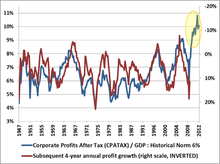
This forecast is also supported by evidence from an analysis of corporate profit margins. In a recent article, John Hussman published a long-term chart of U.S. corporate profits, which demonstrated the magnitude of upward distortion endemic in current corporate profits, which we have reproduced in Chart 1 below. Companies have clearly been benefitting from a period of extraordinary profitability.

Source: John Hussman, 2013

The profit margin picture is critically important. Jeremy Grantham recently stated, "Profit margins are probably the most mean-reverting series in finance, and if profit margins do not mean-revert, then something has gone badly wrong with capitalism. If high profits do not attract competition, there is something wrong with the system and it is not functioning properly." On this basis, we can expect profit margins to begin to revert to more normalized ratios over coming months. If so, stocks may face a future where multiples to corporate earnings are contracting at the same time that the growth in earnings is also contracting. This double feedback mechanism may partially explain why our statistical model predicts such low real returns in coming years. Caveat Emptor.

Modeling Across Many Horizons

Many studies have been published on the Shiller PE, and how well (or not) it estimates future returns. Almost all of these studies apply a rolling 10-year window to earnings as advocated by Dr. Shiller. But is there something magical about a 10-year earnings smoothing factor? Further, is there anything magical about a 10-year forecast horizon?

Kitces (2008, PDF format) demonstrated that "the safe withdrawal rate for a 30-year retirement period has shown a 0.91 correlation to the annualized real return of the portfolio over the first 15 years of the time period". So there is clearly merit in studying a 15-year forecast horizon as well. Further, the tables below will demonstrate that statistical models have the greatest explanatory power at the 15-year horizon.

This study will attempt to address the question of 'perfect forecast horizon', perfect valuation factor, and 'perfect earnings smoothing factor', by analyzing the explanatory power of earnings, the Q-Ratio, and regressed historical stock returns, over return horizons from 1 to 30 years. We will also put all of the factors together to construct an optimized model.

Table 1. below provides a snapshot of some of the results from our analysis. The table shows estimated future returns based on a coherent aggregation of several factor models over some important investment horizons.

Table 1. Factor Based Return Forecasts Over Important Investment Horizons

Source: Shiller (2013), DShort.com (2013), Chris Turner (2013), World Exchange Forum (2013), Federal Reserve (2013), Butler|Philbrick|Gordillo & Associates (2013)

You can see from the table that, according to a model that incorporates valuation estimates from 4 distinct domains, and which explains over 80% of historical returns since 1871, stocks are likely to deliver 1% or less in real total returns over the next 5 to 20 years. Yikes.

Process

The purpose of our analysis was to examine several methods of capturing market valuation to determine which methods were more or less efficacious. Furthermore, we were interested in how to best integrate our valuation metrics into a coherent statistical framework that would provide us with the best estimate of future returns.

Our approach relies on a common statistical technique called linear regression, which takes as inputs the valuation metrics we calculate from a variety of sources, and determines how sensitive actual future returns are to contemporaneous observations of each metric. Linear regression creates a linear function, which by definition can be described by a slope value and an intercept value, which we provide below for each metric and each forecast horizon. A further advantage of linear regression is that we can measure how confident we can be in the estimate provided by the analysis. The quantity we use to measure confidence in the estimates is called the R-Squared.

The following matrices show the R-Squared ratio, regression slope, regression intercept, and current  forecast returns based on a regression analysis for each valuation factor. The matrices are heat-mapped so that larger values are reddish, and small or negative values are blue-ish. Click on each image for a large version.

Matrix 1. Explanatory power of valuation/future returns relationships

Source: Shiller (2013), DShort.com (2013), Chris Turner (2013), World Exchange Forum (2013), Federal Reserve (2013), Butler|Philbrick|Gordillo & Associates (2013)

Matrix 1. contains a few important observations. Notably, over periods of 10-20 years, the Q ratio, very long-term smoothed PE ratios, and market capitalization / GNP ratios are equally explanatory, with R-Squared ratios around 55%.  The best estimate (perhaps tautologically given the derivation) is derived from the price residuals, which simply quantify how extended prices are above or below their long-term trend.

The worst estimates are those derived from trailing 12-month PE ratios (PE1 in Matrix 1 above). Many analysts quote 'Trailing 12-Months' or TTM PE ratios for the market as a tool to assess whether markets are cheap or expensive. If you hear an analyst quoting the market's PE ratio, odds are they are referring to this TTM number. Our analysis slightly modifies this measure by averaging the PE over the prior 12 months rather than using trailing cumulative earnings through the current month, but this change does not substantially alter the results.

As it turns out, TTM (or PE1) Price/Earnings ratios offer the least information about subsequent returns relative to all of the other metrics in our sample. As a result, investors should be extremely skeptical of conclusions about market return prospects presented by analysts who justify their forecasts based on trailing 12-month ratios.

Forecasting Expected Returns

We expect you to be skeptical of our unconventional assertions, so below we provide the precise calculations we used to determine our estimates. The following matrices provide the slope and intercept coefficients for each regression. We have provided these in order to illustrate how we calculated the values for the final matrix below of predicted future returns to stocks.

Matrix 2. Slope of regression line for each valuation factor/time horizon pair.

Source: Shiller (2013), DShort.com (2013), Chris Turner (2013), World Exchange Forum (2013), Federal Reserve (2013), Butler|Philbrick|Gordillo & Associates (2013)

Matrix 3. Intercept of regression line for each valuation factor/time horizon pair.

Source: Shiller (2013), DShort.com (2013), Chris Turner (2013), World Exchange Forum (2013), Federal Reserve (2013), Butler|Philbrick|Gordillo & Associates (2013)

Matrix 4. shows forecast future real returns over each time horizon, as calculated from the slopes and intercepts above, by using the most recent values for each valuation metric (through February 2013). 

For statistical reasons which are beyond the scope of this study, when we solve for future returns based on current monthly data, we utilize the rank in the equation for each metric, not the nominal value.

For example, the 15-year return forecast based on the current Q-Ratio can be calculated by multiplying the current ordinal rank of the Q-Ratio (1171) by the slope from Matrix 2. at the intersection of 'Q-Ratio' and '15-Year Rtns' (-0.000086098), and then adding the intercept at the same intersection (0.119607) from Matrix 3. The result is 0.0188, or 1.88%, as you can see in Matrix 4. below at the same intersection (Q-Ratio | 15-Year Rtns).

Matrix 4. Modeled forecast future returns using current valuations.

Source: Shiller (2013), DShort.com (2013), Chris Turner (2013), World Exchange Forum (2013), Federal Reserve (2013), Butler|Philbrick|Gordillo & Associates (2013)

Finally, at the bottom of the above matrix we show the forecast returns over each future horizon based on our best-fit multiple regression from the factors above. From the matrix, note that the best forecast for future real equity returns integrating all available valuation metrics is 1% or less per year over horizons covering the next 5 to 20 years. We also provided the R-squared for each multiple regression underneath each forecast; you can see that at the 15-year forecast horizon, our regression explains 80% of total returns to stocks.

Chart 2. below demonstrates how closely the model tracks actual future 15-year returns. The red line tracks the model's forecast annualized real total returns over subsequent 15-year periods using our best fit multiple regression model . The blue line shows the actual annualized real total returns over the same 15-year horizon.

Chart 2. 15-Year Forecast Returns vs. 15-Year Actual Future Returns

Source: Shiller (2011), DShort.com (2011), Chris Turner (2011), World Exchange Forum (2011), Federal Reserve (2011), Butler|Philbrick & Associates (2011)

You can see that 15-year "Regression Forecast" returns are -0.43% per year  using market valuations as of February 28, 2013.

Putting the Predictions to the Test

A model is not very interesting or useful unless it actually does a good job of predicting the future. To that end, we tested the model's predictive capacity at some key turning points in markets over the past century or more to see how well it predicted future inflation-adjusted returns.

Table 2. Comparing Long-term average forecasts with model forecasts

Source: Shiller (2013), DShort.com (2013), Chris Turner (2013), World Exchange Forum (2013), Federal Reserve (2013), Butler|Philbrick|Gordillo & Associates (2013)

You can see we tested against periods during the Great Depression, the 1970s inflationary bear market, the 1982 bottom, and the middle of the 1990s technology bubble in 1995. The table also shows expected 15-year returns given market valuations at the 2009 bottom, and current levels. These are shaded green because we do not have 15-year future returns from these periods yet.

Observe that, at the very bottom of the bear market in 2009, real total return forecasts never edged higher than 7%, which is only slightly above the long-term average return. This suggests that prices just approached fair value at the market's bottom; they were nowhere near the level of cheapness that markets achieved at bottoms in 1932 or 1982. As of the end of February 2013, annualized future returns over the next 15 years are expected to be less than 0 percent.

We compared the forecasts from our model with what would be expected from using just the long-term average real returns of 6.5% as a constant forecast, and demonstrated that always using the long-term average return as the future return estimate resulted in 350% more error than estimations from our multi-factor regression model over 15-year forecast horizons (1.22% annualized return error from our model vs 5.55% using the long-term average). Clearly the model offers substantially more insight into future return expectations than simple long-term averages, especially near valuation extremes.

Conclusions

The 'Regression Forecast' return predictions along the bottom of Matrix 4. are robust predictions for future stock returns, as they account for over 100 different cuts of the data, using 4 distinct valuation techniques, and utilize the most explanatory statistical relationships. The models explain up to 82% of future returns based on R-Squared, and are statistically significant at p~0. Despite the model's robustness over longer horizons, it is critical to note that even this model has very little explanatory power over horizons less than 6 or 7 years, so the model should not be used as a short-term market-timing tool.

Returns in the reddish row labeled "PE1" in Matrix 4 were forecast using just the most recent 12 months of earnings data, and correlate strongly with common "Trailing 12-Month" PE ratios cited in the media. Matrix 1. demonstrates that this trailing 12 month measure is not worth very much as a measure for forecasting future returns over any horizon. However, the more constructive results from this metric probably helps to explain the general consensus among sell-side market strategists that markets will do just fine over coming years.

Just remember that these analysts have no proven ability whatsoever to predict market returns (see here, here, and here). This reality probably has less to do with the analytical ability of most analysts, and more to do with the fact that most clients would choose to avoid investing in stocks altogether if they were told to expect negative real returns over the long-term from high valuations.

Investors would do much better to heed the results of robust statistical analyses of actual market history, and play to the relative odds. This analysis suggests that markets are currently expensive, and asserts a very high probability of low returns to stocks (and possibly other asset classes) in the future. Remember, any returns earned above the average are necessarily earned at someone else's expense, so it will likely be necessary to do something radically different than everyone else to capture excess returns going forward.

Those investors who are determined to achieve long-term financial objectives should be heavily motivated to seek alternatives to traditional investment options given the grim prospects outlined above. Such investors may find solace in some of the approaches related to 'tactical alpha' that we have described in a variety of prior articles.